pacman::p_load(treemap, treemapify, tidyverse) Hands-on Exercise 9.5 - Treemap Visualisation with R
1.Overview
In this hands-on exercise, we explore designing treemaps using R. The exercise consists of three sections: first, manipulating transaction data into a treemap structure using dplyr; second, plotting static treemaps with the treemap package; and third, creating interactive treemaps with the d3treeR package.
2.Installing and Launching R Packages
The code chunk below loads treemap, treemapify and tidyverse into R environment.
3.Data Wrangling
In this exercise, REALIS2018.csv data will be used. This dataset, extracted from REALIS portal, provides information of private property transaction records in 2018.
3.1.Importing the data set
The code chunk below uses read_csv() of readr to import realis2018.csv into R as a tibble data frame called realis2018.
realis2018 <- read_csv("data/realis2018.csv")3.2.Data Wrangling and Manipulation
The realis2018 dataset is in transaction record format, which is too disaggregated for treemap visualization. To prepare it, we will:
Group records by Project Name, Planning Region, Planning Area, Property Type, and Type of Sale.
Compute Total Units Sold, Total Area, Median Unit Price, and Median Transacted Price using appropriate summary statistics.
This transformation is performed using dplyr functions:
group_by()to create groups based on specified variables.summarise()to compute aggregated values for each group.
3.3.Grouped summaries without the Pipe
The code chunk below shows a typical two lines code approach to perform the steps.
realis2018_grouped <- group_by(realis2018, `Project Name`,
                               `Planning Region`, `Planning Area`,
                               `Property Type`, `Type of Sale`)
realis2018_summarised <- summarise(realis2018_grouped,
                          `Total Unit Sold` = sum(`No. of Units`, na.rm = TRUE),
                          `Total Area` = sum(`Area (sqm)`, na.rm = TRUE),
                          `Median Unit Price ($ psm)` = median(`Unit Price ($ psm)`, na.rm = TRUE),
`Median Transacted Price` = median(`Transacted Price ($)`, na.rm = TRUE))Note: Aggregation functions such as sum() and median() obey the usual rule of missing values: if there’s any missing value in the input, the output will be a missing value. The argument na.rm = TRUE removes the missing values prior to computation.
The code chunk above is not very efficient because we have to give each intermediate data.frame a name.
3.4.Grouped summaries with the pipe
The code chunk below shows a more efficient way to tackle the same processes by using the pipe, |>.
realis2018_summarised <- realis2018 |>
  group_by(`Project Name`,`Planning Region`,
           `Planning Area`, `Property Type`,
           `Type of Sale`) |>
  summarise(`Total Unit Sold` = sum(`No. of Units`, na.rm = TRUE),
            `Total Area` = sum(`Area (sqm)`, na.rm = TRUE),
            `Median Unit Price ($ psm)` = median(`Unit Price ($ psm)`, na.rm = TRUE),
            `Median Transacted Price` = median(`Transacted Price ($)`, na.rm = TRUE))
4.Designing Treemap with treemap Package
The treemap package in R is specifically designed for creating highly customizable treemaps. The core function, treemap(), provides extensive flexibility with over 43 arguments. This section focuses on key parameters to create elegant and accurate treemaps.
4.1.Designing a static treemap
To visualize the distribution of median unit prices and total units sold for resale condominiums by geographic hierarchy in 2017, we follow these steps:
Filter the Data: Select only records related to resale condominiums from the
realis2018_selecteddataset.Use
treemap(): Generate the treemap with appropriate arguments to represent median unit prices and total units sold.
realis2018_selected <- realis2018_summarised %>%
  filter(`Property Type` == "Condominium", `Type of Sale` == "Resale")
4.2.Using the basic arguments
The code chunk below designed a treemap by using 3 core arguments of treemap(), namely: index, vSize and vColor.
treemap(realis2018_selected,
        index=c("Planning Region", "Planning Area", "Project Name"),
        vSize="Total Unit Sold",
        vColor="Median Unit Price ($ psm)",
        title="Resale Condominium by Planning Region and Area, 2017",
        title.legend = "Median Unit Price (S$ per sq. m)"
        )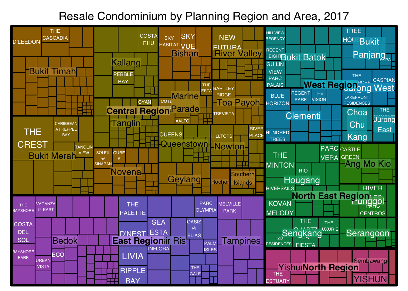
Key takeaways from the 3 arguments used:
index(Hierarchy Definition)This argument defines the hierarchical structure of the treemap.
It must contain at least two column names; otherwise, the treemap will not reflect a hierarchy.
The first column represents the highest aggregation level, the second represents the next level, and so on.
vSize(Rectangle Size)This column defines the size of each rectangle in the treemap.
It must contain only non-negative values since the rectangle size is based on numerical scaling.
In our case,
Total Units Soldis a suitable choice forvSize.
vColor(Color Mapping)Important: The default color assignment in
treemap()may not be meaningful.The
vColorargument must be used in combination withtypeto ensure correct color representation.Without explicitly defining
type,treemap()assumestype = "index", which colors the rectangles based on categorical groupings (e.g., planning areas).To properly visualize numerical differences, set
type = "value"and choose a numeric column forvColor(e.g.,Median Unit Price).
4.3.Working with vColor and type arguments
In the code chunk below, type argument is define as value.
treemap(realis2018_selected,
        index=c("Planning Region", "Planning Area", "Project Name"),
        vSize="Total Unit Sold",
        vColor="Median Unit Price ($ psm)",
        type = "value",
        title="Resale Condominium by Planning Region and Area, 2017",
        title.legend = "Median Unit Price (S$ per sq. m)"
        )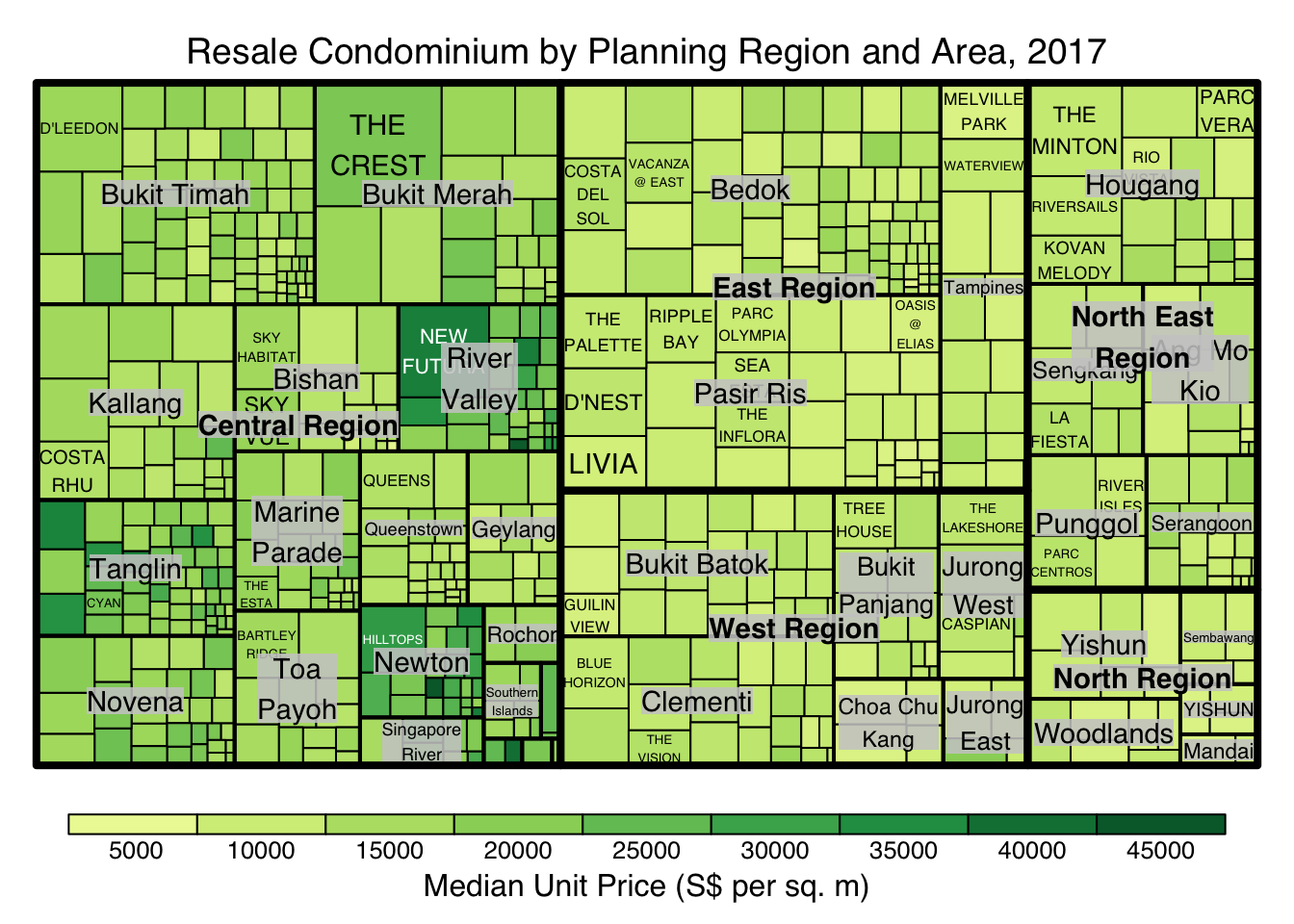
Key Takeaways:
Rectangles are shaded in varying intensities of green, representing median unit prices.
The legend bins values into ten equal intervals (e.g., 0-5000, 5000-10000, etc.).
4.4.Colours in treemap package
mapping & palette: Define how colors are assigned.
“value” mapping: Uses a diverging palette (e.g., “RdYlBu”), centering 0 at a neutral color.
“manual” mapping: Maps min to the left, max to the right, and the midpoint to a middle color.
4.5.The “value” type treemap
The code chunk below shows a value type treemap.
treemap(realis2018_selected,
        index=c("Planning Region", "Planning Area", "Project Name"),
        vSize="Total Unit Sold",
        vColor="Median Unit Price ($ psm)",
        type="value",
        palette="RdYlBu",
        title="Resale Condominium by Planning Region and Area, 2017",
        title.legend = "Median Unit Price (S$ per sq. m)"
        )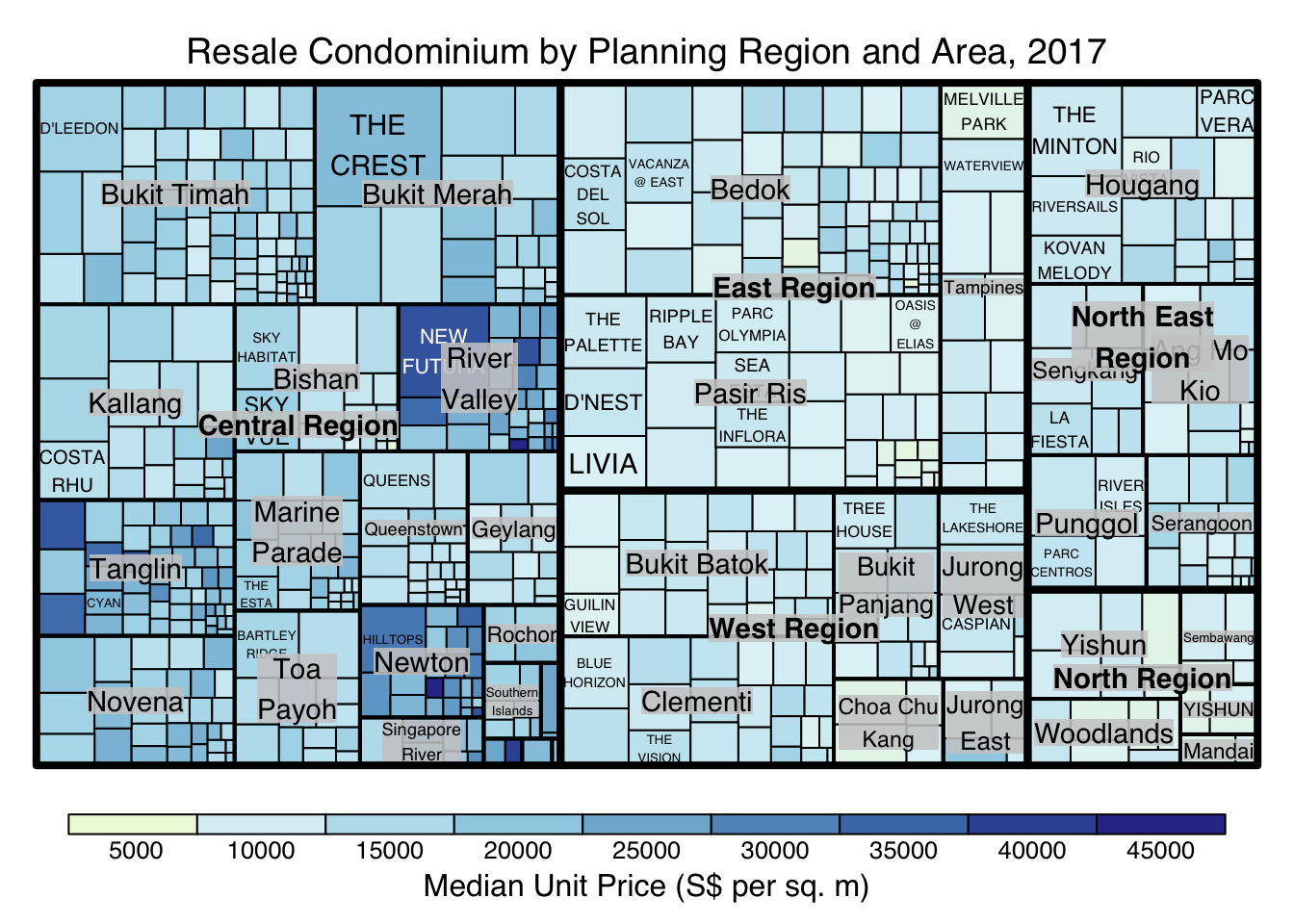
Key takeaways from the above code chunk:
No red rectangles appear in the RdYlBu palette because all median unit prices are positive.
The legend shows 5000 to 45000 due to default range settings, which adjust to min and max values with rounding.
4.6.The “manual” type treemap
The “manual” type does not interpret the values as the “value” type does. Instead, the value range is mapped linearly to the colour palette.
The code chunk below shows a manual type treemap.
treemap(realis2018_selected,
        index=c("Planning Region", "Planning Area", "Project Name"),
        vSize="Total Unit Sold",
        vColor="Median Unit Price ($ psm)",
        type="manual",
        palette="RdYlBu",
        title="Resale Condominium by Planning Region and Area, 2017",
        title.legend = "Median Unit Price (S$ per sq. m)"
        )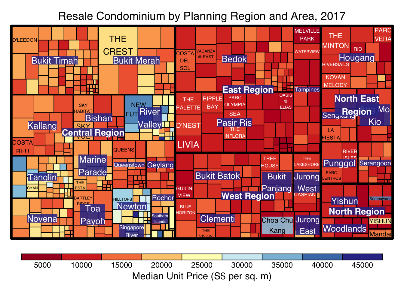
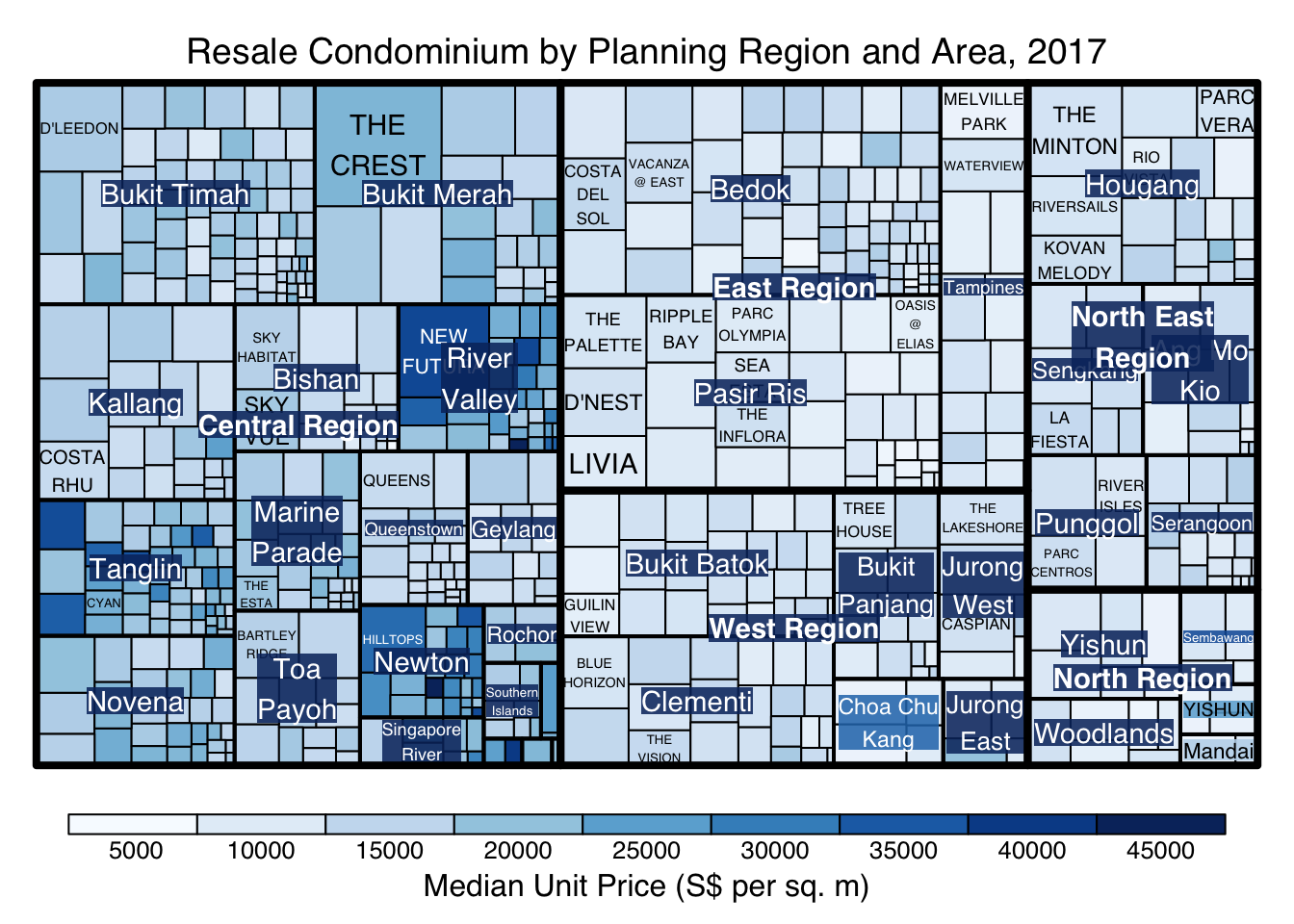
The colour scheme used is very copnfusing, as mapping = (min(values), mean(range(values)), max(values)). It is not wise to use diverging colour palette such as RdYlBu if the values are all positive or negative.
To overcome this problem, a single colour palette such as Blues should be used.
treemap(realis2018_selected,
        index=c("Planning Region", "Planning Area", "Project Name"),
        vSize="Total Unit Sold",
        vColor="Median Unit Price ($ psm)",
        type="manual",
        palette="Blues",
        title="Resale Condominium by Planning Region and Area, 2017",
        title.legend = "Median Unit Price (S$ per sq. m)"
        )
4.7.Treemap Layout
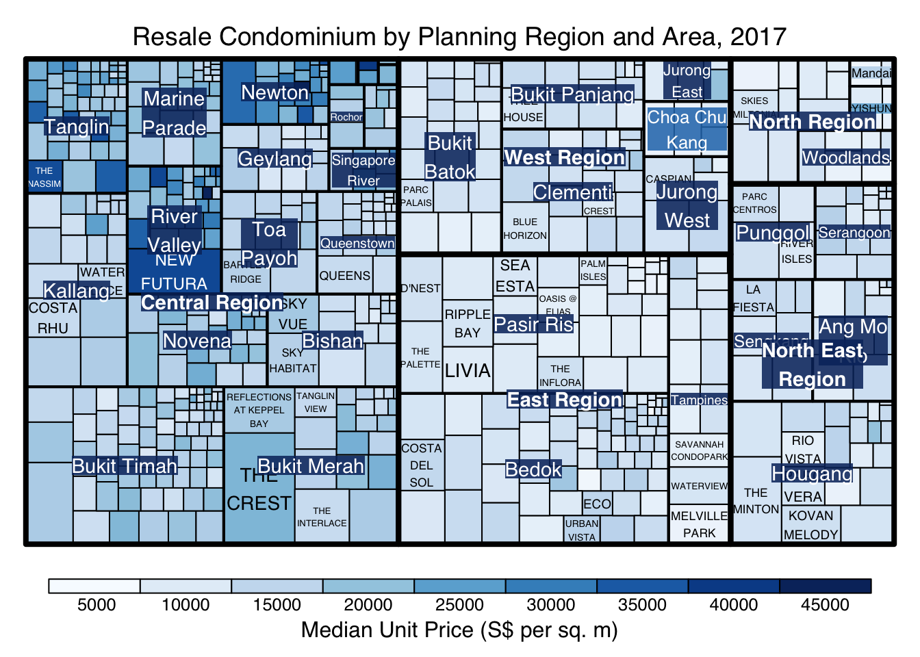
treemap() supports two layouts: squarified (optimizes aspect ratios but ignores sorting) and pivot-by-size (maintains sorting with acceptable aspect ratios). The default is pivot-by-size.
4.8.Working with algorithm argument
The code chunk below plots a squarified treemap by changing the algorithm argument.
treemap(realis2018_selected,
        index=c("Planning Region", "Planning Area", "Project Name"),
        vSize="Total Unit Sold",
        vColor="Median Unit Price ($ psm)",
        type="manual",
        palette="Blues",
        algorithm = "squarified",
        title="Resale Condominium by Planning Region and Area, 2017",
        title.legend = "Median Unit Price (S$ per sq. m)"
        )
4.9.Using sortID
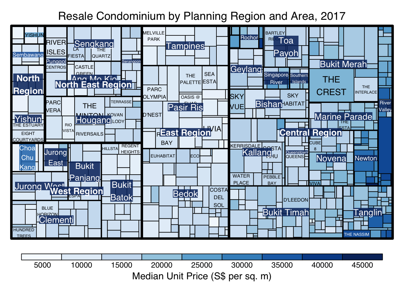
When “pivotSize” algorithm is used, sortID argument can be used to dertemine the order in which the rectangles are placed from top left to bottom right.
treemap(realis2018_selected,
        index=c("Planning Region", "Planning Area", "Project Name"),
        vSize="Total Unit Sold",
        vColor="Median Unit Price ($ psm)",
        type="manual",
        palette="Blues",
        algorithm = "pivotSize",
        sortID = "Median Transacted Price",
        title="Resale Condominium by Planning Region and Area, 2017",
        title.legend = "Median Unit Price (S$ per sq. m)"
        )
5.Designing Treemap using treemapify Package
treemapify is a R package specially developed to draw treemaps in ggplot2. In this section, we explore how to design treemps closely resemble those in previous section using treemapify. Before getting started, you should read Introduction to “treemapify” its user guide.
5.1.Designing a basic treemap
ggplot(data=realis2018_selected,
       aes(area = `Total Unit Sold`,
           fill = `Median Unit Price ($ psm)`),
       layout = "scol",
       start = "bottomleft") +
  geom_treemap() +
  scale_fill_gradient(low = "light blue", high = "blue")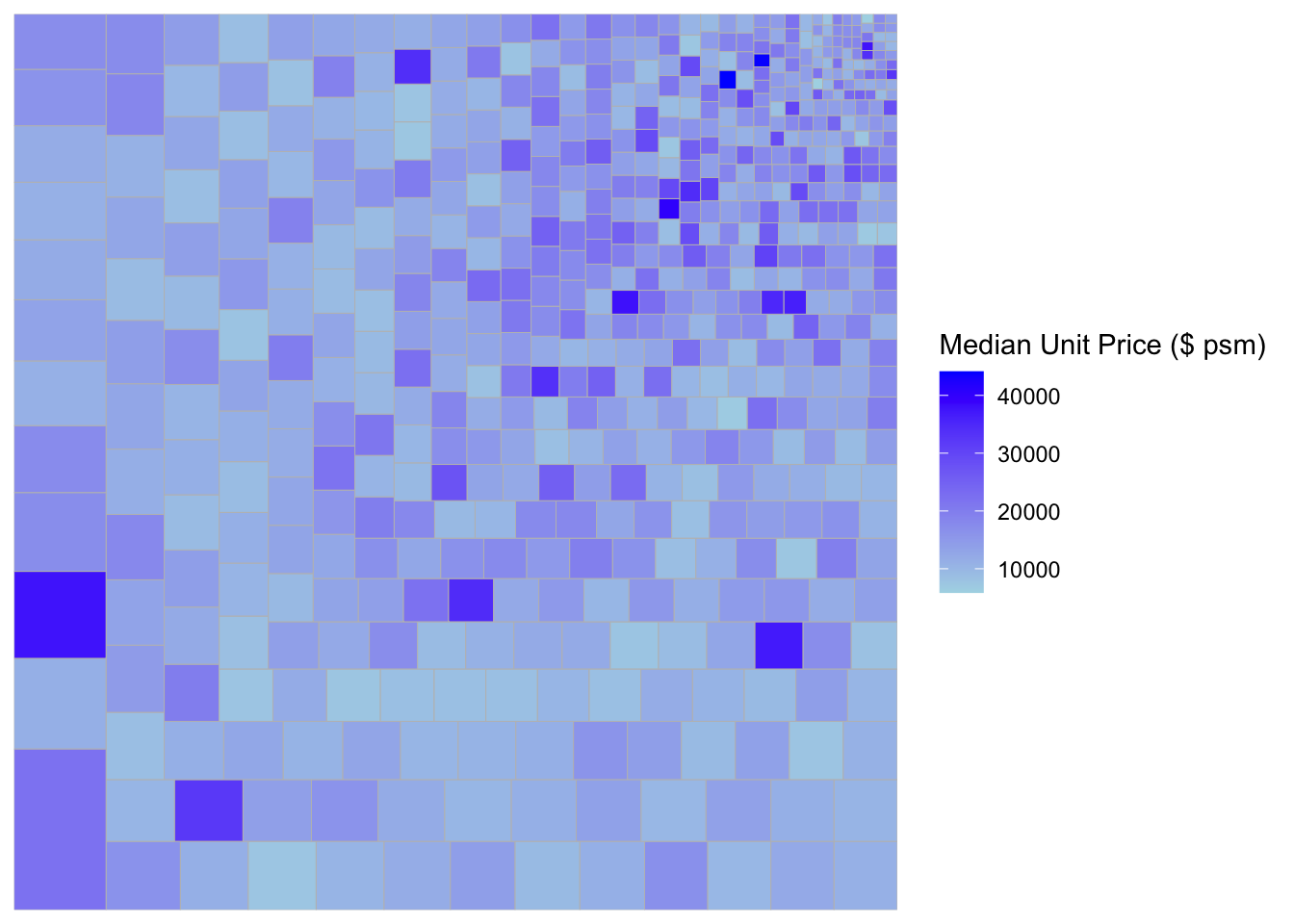
5.2.Defining hierarchy
Group by Planning Region
ggplot(data=realis2018_selected,
       aes(area = `Total Unit Sold`,
           fill = `Median Unit Price ($ psm)`,
           subgroup = `Planning Region`),
       start = "topleft") +
  geom_treemap()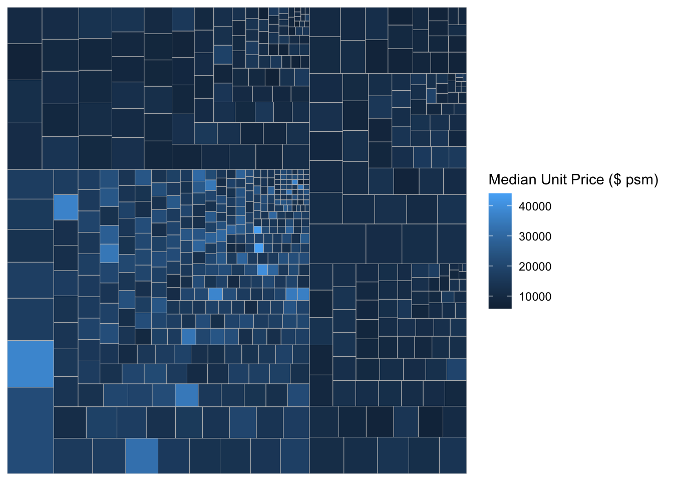
Group by Planning Area
ggplot(data=realis2018_selected,
       aes(area = `Total Unit Sold`,
           fill = `Median Unit Price ($ psm)`,
           subgroup = `Planning Region`,
           subgroup2 = `Planning Area`)) +
  geom_treemap()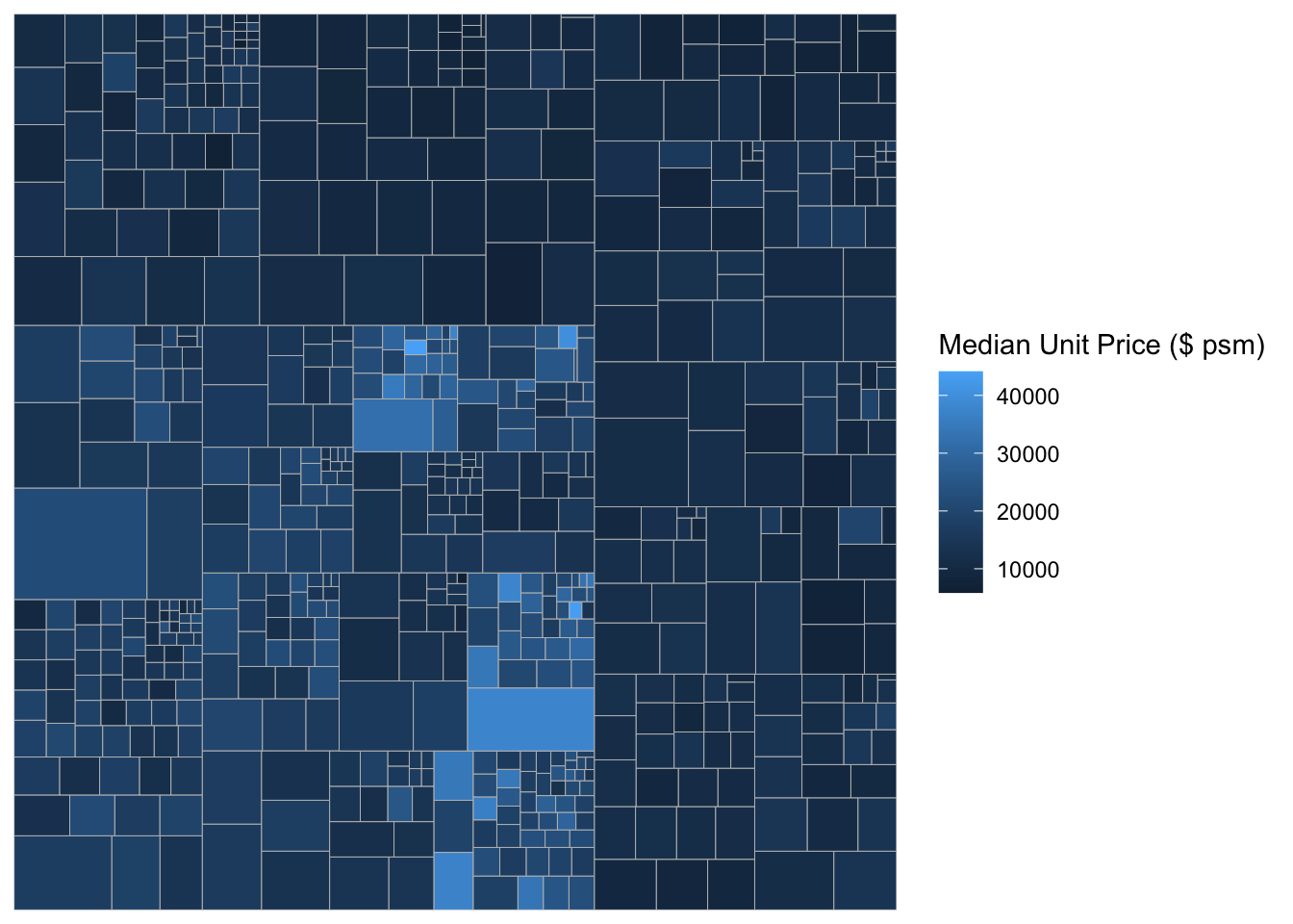
Adding boundary line
ggplot(data=realis2018_selected,
       aes(area = `Total Unit Sold`,
           fill = `Median Unit Price ($ psm)`,
           subgroup = `Planning Region`,
           subgroup2 = `Planning Area`)) +
  geom_treemap() +
  geom_treemap_subgroup2_border(colour = "gray40",
                                size = 2) +
  geom_treemap_subgroup_border(colour = "gray20")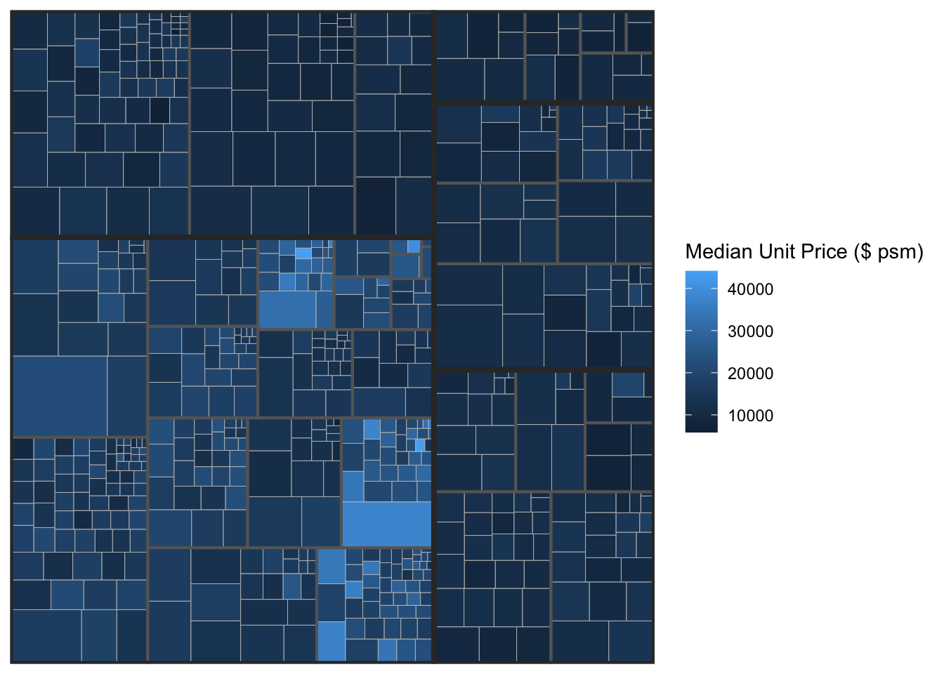
6.Designing Interactive Treemap using d3treeR
6.1.Installing d3treeR package
This sections shows you how to install a R package which is not available in cran.
If this is the first time you install a package from github, you should install devtools package by using the code below or else you can skip this step.
install.packages("devtools")Next, you will load the devtools library and install the package found in github by using the codes below.
library(devtools)
install_github("timelyportfolio/d3treeR")
Now you are ready to launch d3treeR package
library(d3treeR)6.2.Designing An Interactive Treemap
The codes below perform two processes.
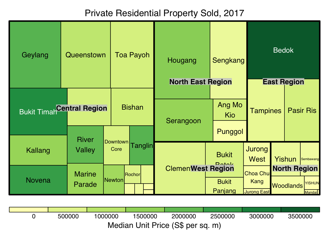
Firsttreemap() is used to build a treemap using selected variables in realis2018_summarised data.frame. The treemap created is save as object called tm.
tm <- treemap(realis2018_summarised,
        index=c("Planning Region", "Planning Area"),
        vSize="Total Unit Sold",
        vColor="Median Unit Price ($ psm)",
        type="value",
        title="Private Residential Property Sold, 2017",
        title.legend = "Median Unit Price (S$ per sq. m)"
        )
Then d3tree() is used to build an interactive treemap.
d3tree(tm,rootname = "Singapore" )