In-class Exercise 5

1. Getting Started

1.1. Loading Packages

In the code chunk below, p_load() of pacman package is used to load the R packages into R environment

pacman::p_load(tidyverse, jsonlite,
               SmartEDA, tidygraph,
               ggraph)

1.2. Importing JSON

In the code chunk, fromJSON() of jsonlite package is used to import MC1_graph.json file into R and save the output subject

kg <- fromJSON("data/MC1_graph.json")

1.3. Inspecting structure

str(kg, max.level = 1)

List of 5
 $ directed  : logi TRUE
 $ multigraph: logi TRUE
 $ graph     :List of 2
 $ nodes     :'data.frame': 17412 obs. of  10 variables:
 $ links     :'data.frame': 37857 obs. of  4 variables:

1.4. Extracting and inspecting

nodes_tbl <- as_tibble(kg$nodes)
edges_tbl <- as_tibble(kg$links)

2. Initial EDA

2.1. Edge Type

ggplot(data = edges_tbl, 
       aes(y = `Edge Type`, fill = `Edge Type`)) +
  geom_bar()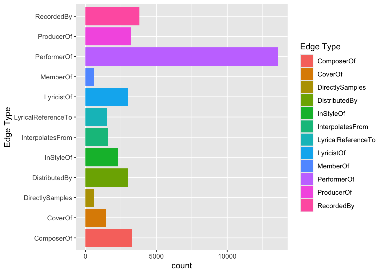

2.2. Node Type

ggplot(data = nodes_tbl, 
       aes(y = `Node Type`, fill = `Node Type`)) +
  geom_bar()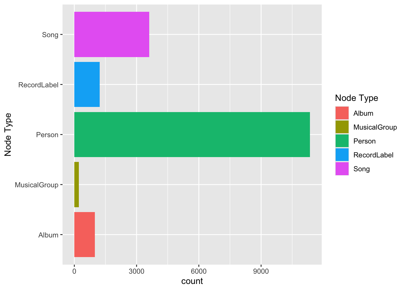

3. Creating Knowledge Graph

3.1. Step 1: Mapping from node ID to row Index

id_map <- tibble(id=nodes_tbl$id,
                 index = seq_len(nrow(nodes_tbl)))

This ensures each id from your node list is mapped to the correct row number.

3.2. Step 2: Map source and target IDs to row indices

edges_tbl <- edges_tbl %>%
  left_join(id_map, by = c("source" = "id")) %>%

  rename(from = index) %>%
  left_join(id_map, by = c("target" = "id")) %>%

  rename(to = index)

3.3. Step 3: Filter out any unmatched (invalid) edges

edges_tbl <- edges_tbl %>%
  filter(!is.na(from), !is.na(to))

3.4. Step 4: Creating the graph

Lastly, tbl_graph is used to create tidygraph’s graph object by using the code junk below.

graph <- tbl_graph(nodes = nodes_tbl, 
                   edges = edges_tbl,
                   directed = kg$directed)

4. Visualizing the knowledge graph

set.seed(1234)

4.1. Visualizing the whole graph

ggraph(graph, layout ="fr") + 
  geom_edge_link(aplpha = 0.3, colour = "gray") +
  geom_node_point(aes(color = `Node Type`), size = 4) +
  geom_node_text(aes(label = name), repel = TRUE, size = 2.5) +
  theme_void()

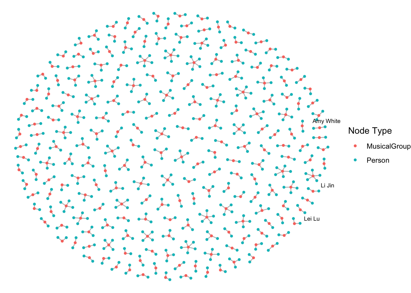
4.2. Visualizing the sub-graph

In this section, we are interested to create a sub-graph based on MemberOf value in Edge_Type column of the edges column of the edge data frame.

4.2.1. Step 1: Filter edges to only `MemberOf’

graph_memberof <- graph %>%
  activate(edges) %>% 
  filter(`Edge Type` == "MemberOf")

4.2.2. Step 2: Extract only connected nodes (i.e., used in these edges)

used_node_indices <- graph_memberof %>%
  activate(edges) %>%
  as_tibble() %>%
  select(from, to) %>%
  unlist() %>%
  unique()

4.2.3. Step 3: Keep only those nodes

graph_memberof <- graph_memberof %>%
  activate(nodes) %>%
  mutate(row_id = row_number()) %>%
  filter(row_id %in% used_node_indices) %>%
  select(-row_id)

4.2.4. Step 4: Plot the sub-graph

ggraph(graph_memberof, layout = "fr") + 
  geom_edge_link(aplpha = 0.5, colour = "gray") +
  geom_node_point(aes(color = `Node Type`), size = 1) +
  geom_node_text(aes(label = name), repel = TRUE, size = 2.5) +
  theme_void()