library(sf)
library(tidyverse)
library(ggplot2)
library(viridis)
library(plotly)
library(dplyr)
library(tidyr)
library(ggiraph)
library(ggridges)
library(ggtern)Take-home Exercise 1 - Phase 1
1. Overview
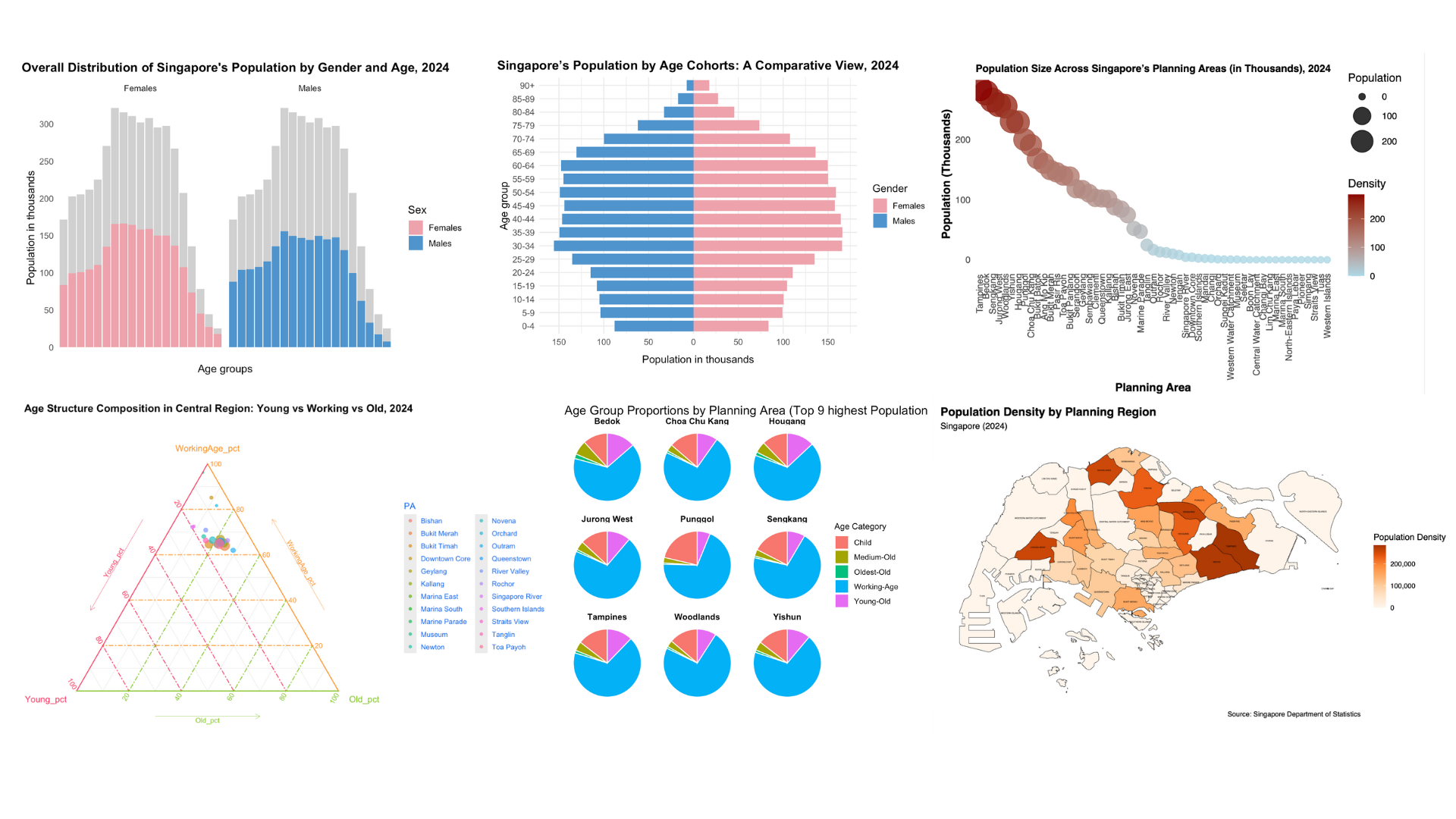
What does Singapore’s population really look like in 2024?
Using interactive visualizations, this article takes you beyond raw numbers to uncover where people live, how age groups are distributed, and which regions are dominated by children, seniors, or working professionals. From balanced age compositions in central districts to extreme skews in lesser-known areas, the charts invite you to explore the evolving face of Singapore — and what it means for the nation’s future.
2. Installing libraries
The required R packages are loaded to provide essential functions for spatial analysis, data manipulation, and visualization.
Note
These libraries collectively support:
- Importing and preparing both tabular and spatial data
- Creating clean, interactive, and informative plots
- Ensuring accessibility through perceptually uniform color palettes
- Enhancing the storytelling aspect of demographic visualizations
3. Importing data
Singapore Residents by Planning Area / Subzone, Single Year of Age and Sex, June 2024 dataset issued by Department of Statistics, Singapore (DOS) is used.
The population dataset for Singapore is imported using the read_csv() function from the readr package.
pop_data <- read_csv("data/singapore_population.csv")📋 Preview of the data:
| PA | SZ | Age | Sex | Pop | Time |
|---|---|---|---|---|---|
| Ang Mo Kio | Ang Mo Kio Town Centre | 0 | Males | 10 | 2024 |
| Ang Mo Kio | Ang Mo Kio Town Centre | 0 | Females | 10 | 2024 |
| Ang Mo Kio | Ang Mo Kio Town Centre | 1 | Males | 10 | 2024 |
| Ang Mo Kio | Ang Mo Kio Town Centre | 1 | Females | 10 | 2024 |
| Ang Mo Kio | Ang Mo Kio Town Centre | 2 | Males | 10 | 2024 |
| Ang Mo Kio | Ang Mo Kio Town Centre | 2 | Females | 10 | 2024 |
The dataset comprises 6 variables and provides detailed demographic information of Singapore’s population in 2024. These variables include:
- Planning Area (PA) and Subzone (SZ), which define the geographical location,
- Age and Sex, which capture demographic attributes,
- Pop, which indicates the population count for each age-sex group within each subzone, and
- Time, which specifies the year of observation.
4. Data Preparation
4.1. Checking missing values and remove if any
The following code snippet checks for missing values in the dataset and calculates the total number and proportion of missing entries:
print(paste('There are ', sum(is.na(data)), ' missing values representing ',
            round(100*sum(is.na(data))/(nrow(data)*ncol(data)), 5), '% of the total.'))
[1] "There are 0 missing values representing % of the total."The dataset contains no missing values. Therefore, no imputation or removal actions are required at this stage.
4.2.Convert Age to Numeric Format
In the dataset, the Age column is not entirely numeric due to the presence of textual values “90_and_Over”. To address this, these values were recoded to “90” using a string replacement function, and the entire column was then converted to numeric format.
pop_data <- pop_data %>%
  mutate(
    Age = str_replace(Age, "^90\\+|90_and_Over", "90"),
    Age = as.numeric(Age)
  )
4.3. Binning Age
a. Into ranges
The continuous Age variable is transformed into categorical age groups. This makes demographic patterns across broader age ranges easier to observe and compare.
age_breaks <- seq(0, 90, by = 5)
age_labels <- c(paste(seq(0, 80, 5), seq(4, 84, 5), sep = "-"), "85-89", "90+")

pop_data <- pop_data %>%
  mutate(
    Age = ifelse(Age == "90+", 90, Age),
    Age = as.numeric(Age),
    AgeGroup = cut(
      Age,
      breaks = c(seq(0, 90, 5), Inf),
      labels = age_labels,
      right = FALSE
    )
  )
b. Into Age categorization
The continuous Age variable is categorized into meaningful demographic age groups. These age bands help standardize population analysis and ensure comparability across studies and time periods.
Note
The age categorization is based on the statistical standards issued by the Singapore Department of Statistics
pop_data <- pop_data %>%
  mutate(
    Age = as.numeric(Age),
    AgeCategory = case_when(
      Age < 15 ~ "Child",
      Age >= 15 & Age < 65 ~ "Working-Age",
      Age >= 65 & Age < 75 ~ "Young-Old",
      Age >= 75 & Age < 85 ~ "Medium-Old",
      Age >= 85 ~ "Oldest-Old"
    )
  )
4.4. Binning Areas into Regional level
To support higher-level geographical analysis, each Planning Area is categorized into a broader Region based on Singapore’s regional classification. This allows for meaningful aggregation, comparison, and visualization of population patterns at the regional level.
Note
The classification follows the official grouping of areas by region as referenced on Wikipedia: Regions of Singapore
pop_data <- pop_data %>%
  mutate(
    Region = case_when(
      PA %in% c("Bishan", "Bukit Merah", "Bukit Timah", "Downtown Core", "Geylang", "Kallang",
                "Marina East", "Marina South", "Marine Parade", "Museum", "Newton", "Novena",
                "Orchard", "Outram", "Queenstown", "Dover", "Ghim Moh", "River Valley", "Rochor",
                "Singapore River", "Southern Islands", "Straits View", "Tanglin", "Toa Payoh") ~ "Central",

      PA %in% c("Bedok", "Changi", "Changi Bay", "Pasir Ris", "Paya Lebar", "Tampines") ~ "East",

      PA %in% c("Central Water Catchment", "Lim Chu Kang", "Mandai", "Sembawang", "Simpang",
                "Sungei Kadut", "Woodlands", "Yishun") ~ "North",

      PA %in% c("Ang Mo Kio", "Hougang", "North-Eastern Islands", "Punggol", "Seletar",
                "Sengkang", "Serangoon") ~ "Northeast",

      TRUE ~ "West"
    )
  )
5. Insight 1: Singapore Population by Gender and Age Group
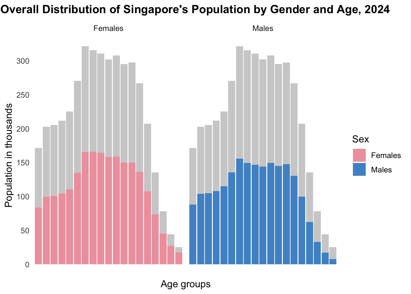
5.2 Insight 1.1: Overall Distribution of Singapore’s Population by Gender and Age, 2024
pop_by_age_gender <- pop_data %>%
  group_by(AgeGroup, Sex) %>%
  summarise(Population = sum(Pop), .groups = "drop")

pop_by_age <- pop_data %>%
  group_by(AgeGroup) %>%
  summarise(Population = sum(Pop), .groups = "drop")

ggplot() +
  geom_bar(data = pop_by_age, aes(x = AgeGroup, y = Population),
           stat = 'identity', alpha = 0.3, fill = 'grey') +
  geom_bar(data = pop_by_age_gender,
           aes(x = AgeGroup, y = Population, fill = Sex),
           stat = 'identity') +
  scale_fill_manual(values = c('Females' = 'lightpink2', 'Males' = 'steelblue3')) +
  facet_grid(~Sex) +
  scale_x_discrete(labels = NULL) +
  scale_y_continuous(
    breaks = c(seq(0, 400000, 50000)),
    labels = c(seq(0, 400, 50))
  ) +
  theme_minimal() +
  ggtitle("Singapore Population by Gender and Age Group, 2024") +
  xlab("Age groups") +
  ylab("Population in thousands")
)- Overall age structure: The grey background bars illustrate the total population across age groups, revealing a skew towards younger cohorts — with over 85% of the population below age 65.
- Females dominance in older age: When comparing gender-specific age structures, it is evident that females have a greater representation in the older age brackets, highlighting higher life expectancy among women.
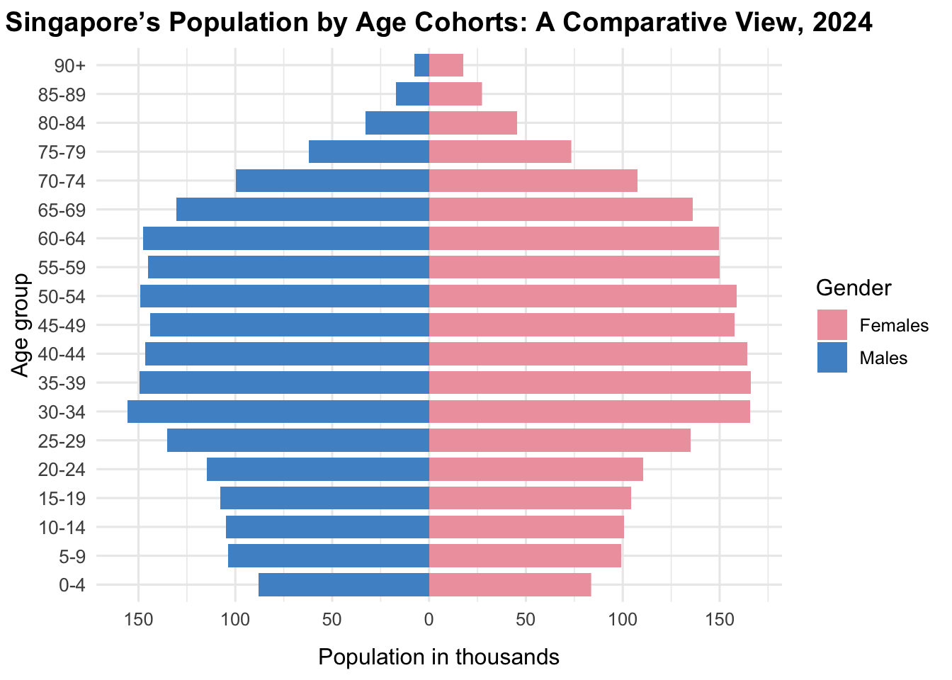
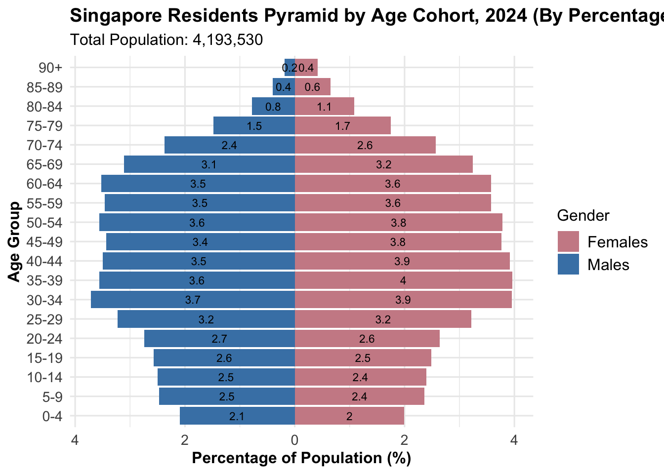
5.3. Insight 1.2. Singapore’s Population by Age Cohorts: A Comparative View
pyramid_data <- pop_data %>%
  mutate(Pop = ifelse(Sex == "Males", -Pop, Pop))

ggplot(pyramid_data, aes(x = AgeGroup, y = Pop, fill = Sex)) +
  geom_bar(stat = "identity", width = 0.8) +
  coord_flip() +
  scale_y_continuous(
    breaks = seq(-150000, 150000, 50000),
    labels = abs(seq(-150, 150, 50))
  ) +
  scale_fill_manual(values = c("Females" = "lightpink2", "Males" = "steelblue3")) +
  labs(
    title = "Singapore Residents Pyramid by Age Cohort, 2024",
    x = "Age group",
    y = "Population in thousands",
    fill = "Gender"
  ) +
  theme_minimal() +
  theme(
    plot.title = element_text(hjust = 0.5, face = "bold"),
    axis.text.y = element_text(size = 10),
    axis.title.x = element_text(margin = margin(t = 10))
)- Working-age concentration: The largest population segments fall within the 25–54 age range, indicating a strong labor force presence.
- Lower birth rate signal: The narrow base (ages 0–14) points to a decline in birth rates, which may pose challenges for future demographic sustainability.
- Balanced young-to-middle age cohorts: From ages 0 to 60, the pyramid shows almost equal numbers of males and females, suggesting balanced gender distribution in most age groups.
- Gender disparity at the top: Starting from age 75 and above, there is a visible tilt toward females, again emphasizing greater longevity among women.
6. Insight 2: Population Structure by Planning Area and Age Group
6.1 Insight 2.1. Population Size Across Singapore’s Planning Areas with Interactivity
pop_summary <- pop_data %>%
  group_by(PA) %>%
  summarise(Pop = sum(Pop) / 1000, .groups = "drop")

p <- ggplot(pop_summary, aes(x = reorder(PA, -Pop), y = Pop)) +
  geom_point_interactive(
    aes(size = Pop, color = Pop,
        tooltip = paste0(PA, "\nPopulation: ", round(Pop, 1), "K"),
        data_id = PA),
    alpha = 0.8
  ) +
  scale_size(range = c(3, 12)) +
  scale_color_gradient(low = "lightblue", high = "darkred") +
  labs(
    title = "Population by Planning Area (in Thousands)",
    x = "Planning Area", y = "Population (Thousands)",
    color = "Density", size = "Population"
  ) +
  theme_minimal() +
  theme(axis.text.x = element_text(angle = 90, vjust = 0.5, hjust = 1))

girafe(ggobj = p)- Tampines, Bedok, and Jurong West are the most populated and dense.
- Western Islands and Tuas have the lowest population and density.
- The population is concentrated in a few key areas.
6.2. Insight 2.2. Population Size Across Singapore (Regional level) with Interactivity
region_summary <- pop_data %>%
  filter(!is.na(Region)) %>%
  group_by(Region) %>%
  summarise(Pop = sum(Pop) / 1000, .groups = "drop")

p <- ggplot(region_summary, aes(x = reorder(Region, -Pop), y = Pop)) +
  geom_point_interactive(
    aes(size = Pop, color = Pop,
        tooltip = paste0(Region, "\nPopulation: ", round(Pop, 1), "K"),
        data_id = Region),
    alpha = 0.8
  ) +
  scale_size(range = c(4, 14)) +
  scale_color_gradient(low = "lightblue", high = "darkred") +
  labs(
    title = "Population by Region (in Thousands)",
    x = "Region", y = "Population (Thousands)",
    color = "Density", size = "Population"
  ) +
  theme_minimal() +
  theme(
    panel.grid = element_blank(),
    axis.text.x = element_text(angle = 0, vjust = 0.5, hjust = 0.5),
    axis.title = element_text(size = rel(1), face = "bold"),
    plot.title = element_text(size = rel(1.2), face = "bold")
  )

girafe(
  ggobj = p,
  width_svg = 7,
  height_svg = 6
)- Northeast, Central, and Other regions have the highest populations, each nearing or exceeding 950K, as shown by their large bubble size and dark color.
- East region follows, with a moderate population around 710K.
- North region has the lowest population, approximately 600K, evident from its smaller, lighter-colored bubble.
6.3. Insight 2.3. Age Structure Composition by Planning Area: Young vs Working vs Old
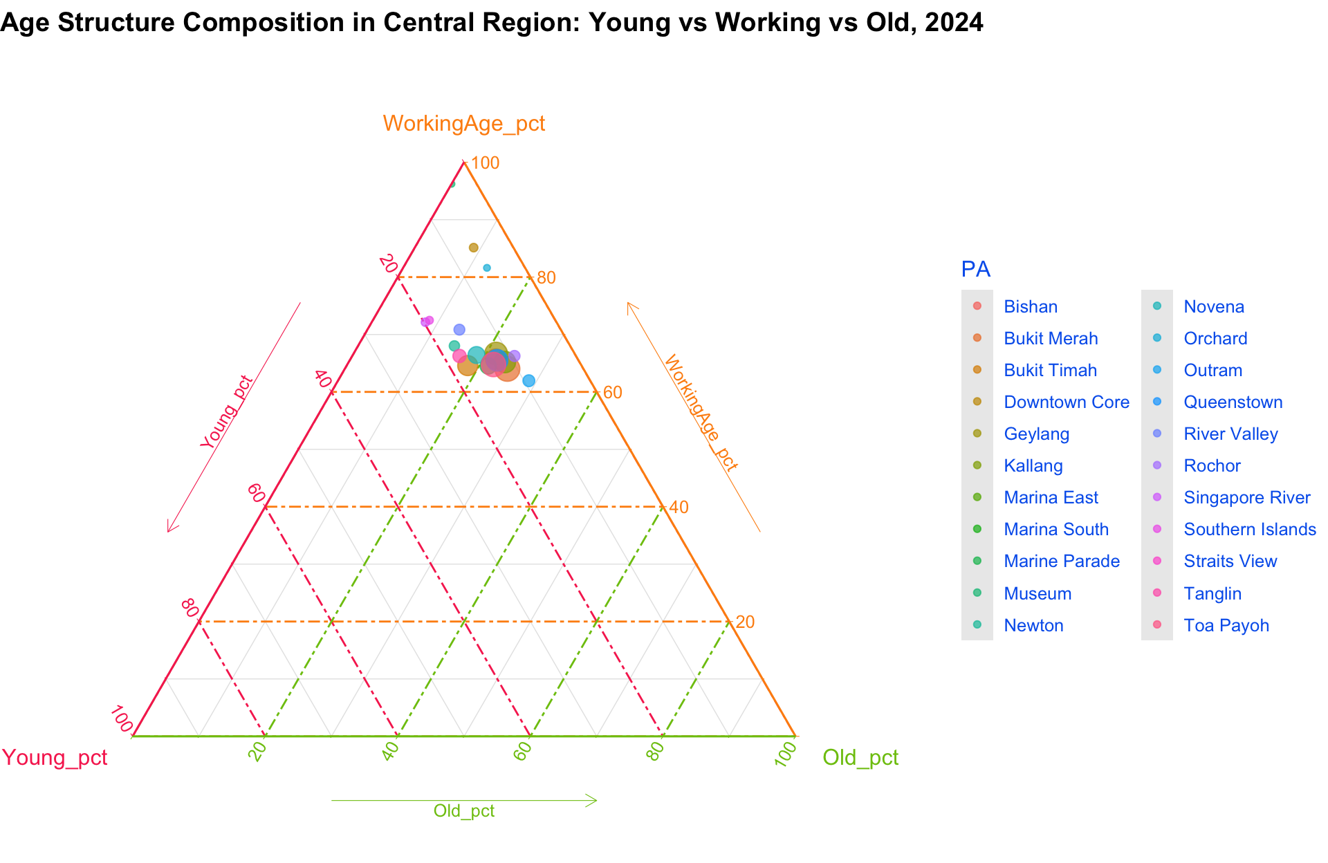
- Diverse distribution: Planning areas in the Central region show a relatively balanced age composition, with most areas clustering near the center of the ternary plot.
- High working-age concentration: Majority of dots tilt toward the WorkingAge corner, suggesting Central areas are hubs for working professionals.
- Moderate ageing: A few areas like Tanglin, Toa Payoh, and Outram lean slightly toward the Old vertex, indicating a notable proportion of elderly residents.
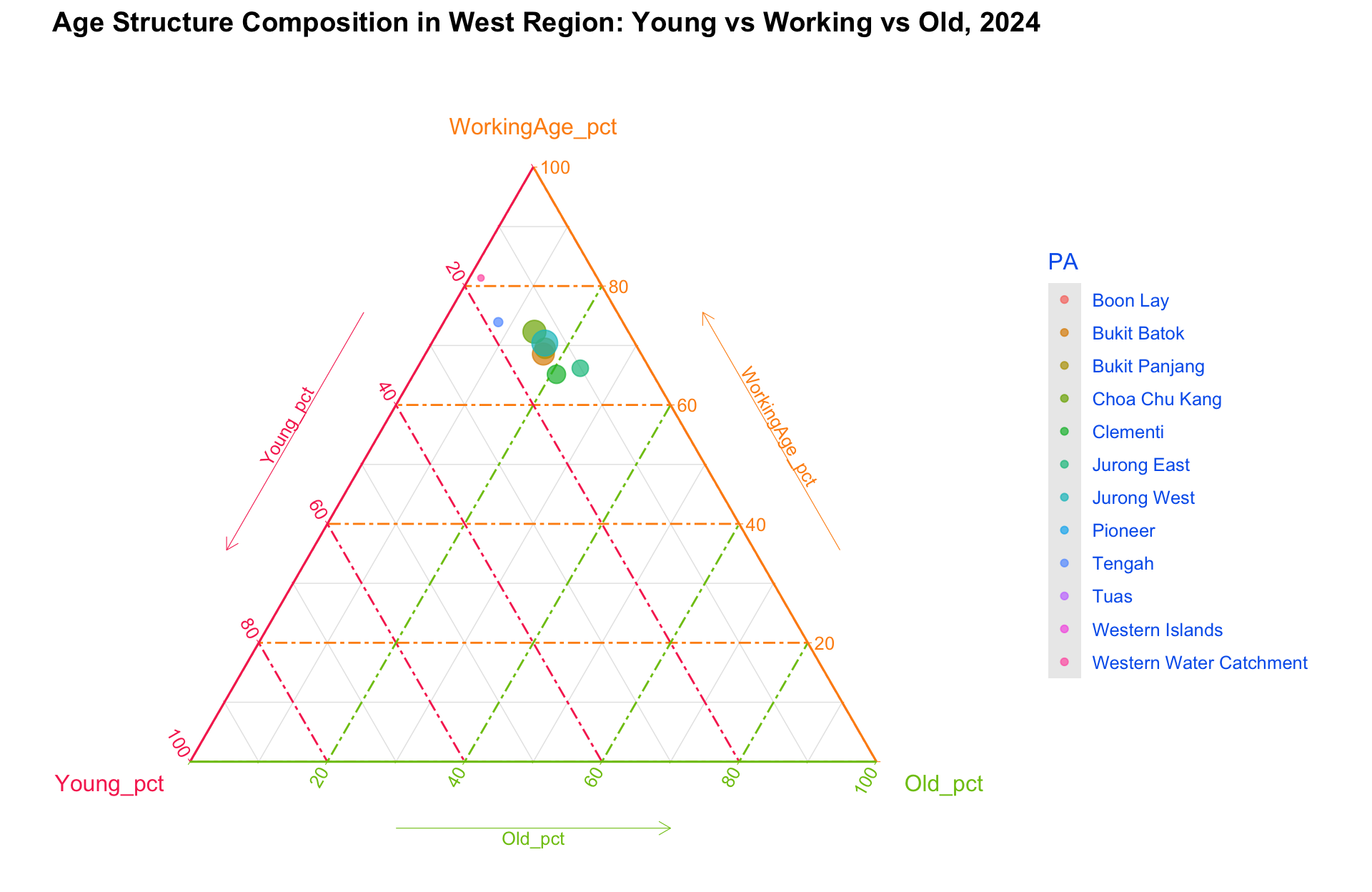
- Young and working-heavy areas: Most planning areas in the West cluster around high WorkingAge and Young proportions.
- Low ageing population: The Old_pct values remain consistently low, pointing to younger families or newer housing developments.
- Urban expansion: Areas like Tengah and Jurong West are reflective of growing, youthful populations driven by infrastructure and development projects.
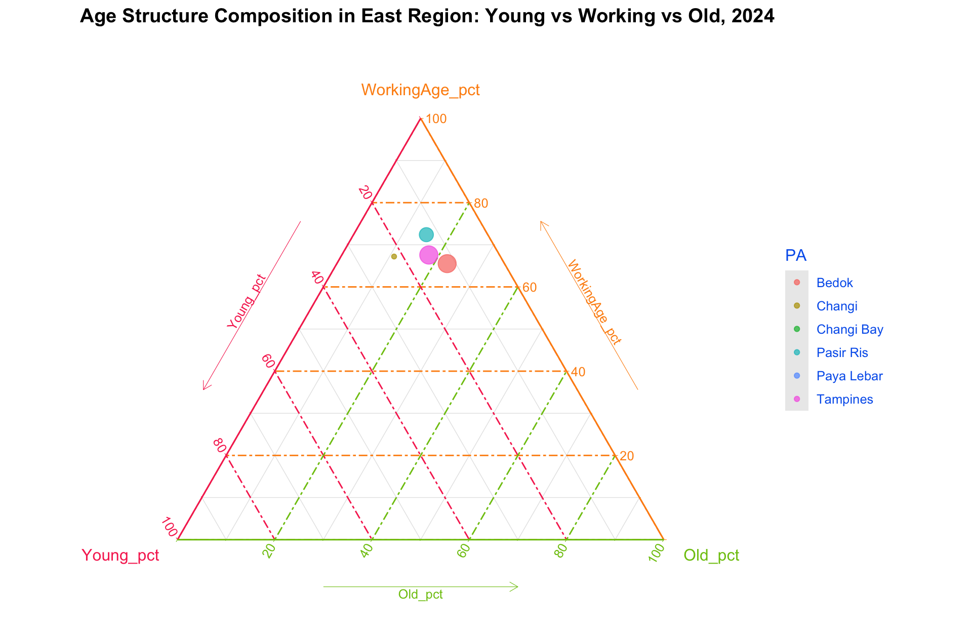
- Even spread: Eastern areas like Tampines and Pasir Ris show more spread between Young and Old, though still strongly working-age dominant.
- Retirement-ready areas : Slight drift toward the Old vertex for Bedok and Paya Lebar could reflect ageing-in-place among long-term residents.
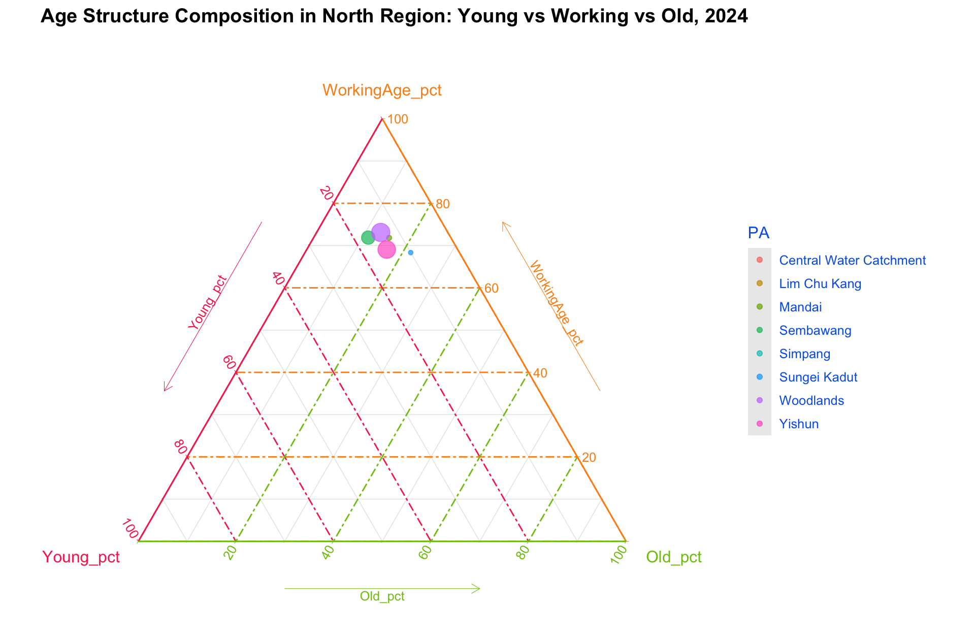
- Compact cluster: Northern areas group tightly near the WorkingAge vertex with low Young and Old percentages, suggesting a middle-aged population base.
- Low youth share: Unlike the West or North-East, Young_pct is relatively lower, possibly due to migration or fewer new housing estates.
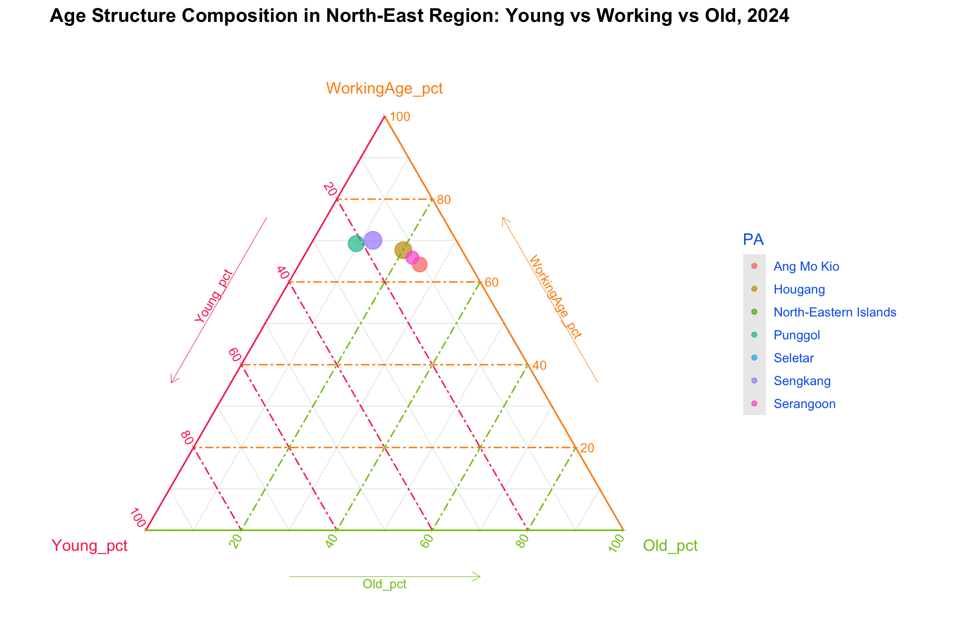
- Youth-oriented mix: Strong presence of Young and WorkingAge populations, especially in areas like Punggol and Sengkang — both known for family-friendly housing.
- Minimal ageing: Most North-East areas have the lowest Old_pct, indicating these are emerging or recently developed neighborhoods with few elderly residents.
ternary_data <- pop_data %>%
  filter(Region == "Northeast" & !is.na(AgeCategory)) %>%
  mutate(AgeGroup = case_when(
    AgeCategory == "Child" ~ "Young",
    AgeCategory == "Working-Age" ~ "WorkingAge",
    AgeCategory %in% c("Young-Old", "Medium-Old", "Oldest-Old") ~ "Old"
  )) %>%
  group_by(PA, AgeGroup) %>%
  summarise(Pop = sum(Pop), .groups = "drop") %>%
  tidyr::pivot_wider(names_from = AgeGroup, values_from = Pop, values_fill = 0) %>%
  mutate(
    Total = Young + WorkingAge + Old,
    Young_pct = Young / Total,
    WorkingAge_pct = WorkingAge / Total,
    Old_pct = Old / Total
  )

ggtern(data = ternary_data,
       aes(x = Young_pct, y = WorkingAge_pct, z = Old_pct,
           color = PA, size = Total)) +
  geom_point(alpha = 0.7) +
  labs(
    title = "Age Structure Composition in North-East Region: Young vs Working vs Old, 2024"
  ) +
  theme_tropical() +
  guides(size = "none") +
  theme(
    legend.position = "right",
    legend.justification = "center",
    legend.direction = "vertical",
    plot.title = element_text(hjust = 0.5)
  )
Replace Region == ' ' by Central, East, West, North-East, North, respectively
6.4. Insight 2.4. Age Distribution in the Top 9 Most and Least Populated Areas
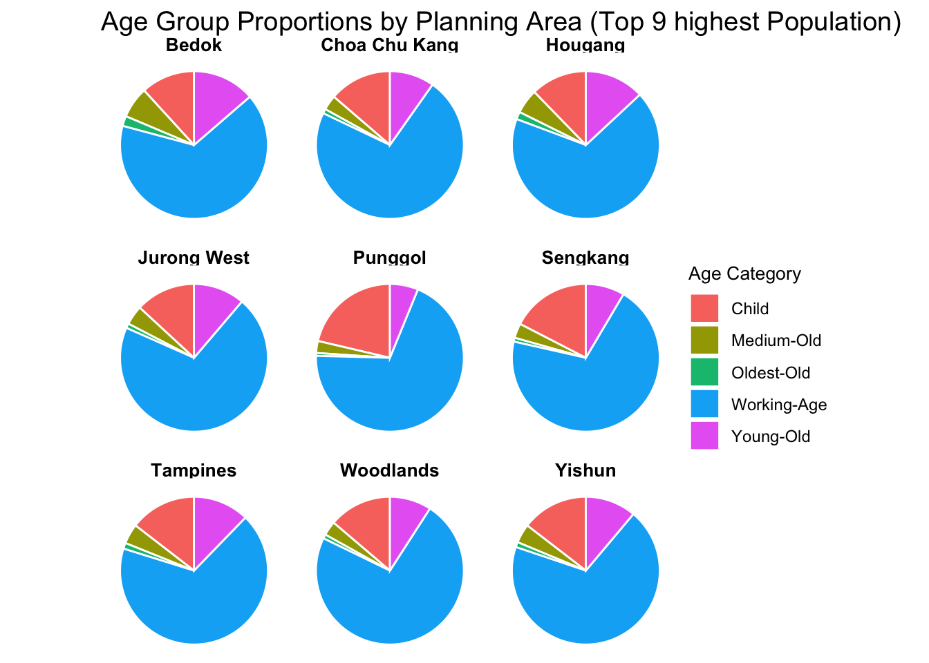
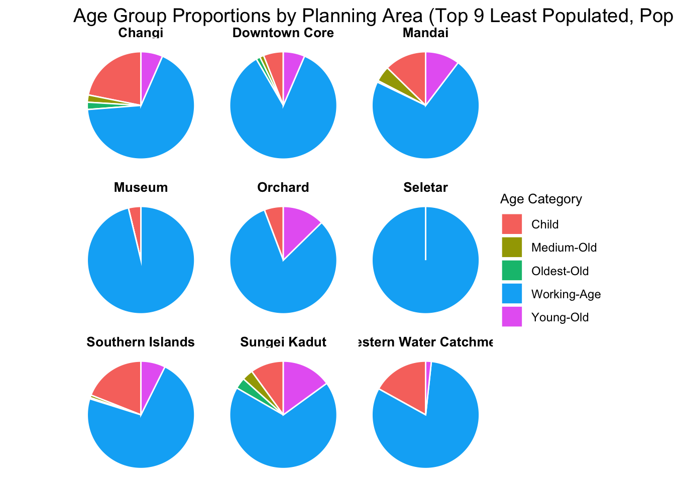
The comparison between the top 9 most and least populated planning areas in Singapore reveals distinct demographic patterns:
a. Top 9 highest population
top9_pa <- pop_data %>%
  filter(!is.na(PA)) %>%
  group_by(PA) %>%
  summarise(Total = sum(Pop), .groups = "drop") %>%
  slice_max(order_by = Total, n = 9) %>%
  pull(PA)


agecat_pct <- pop_data %>%
  filter(PA %in% top9_pa, !is.na(AgeCategory)) %>%
  group_by(PA, AgeCategory) %>%
  summarise(Pop = sum(Pop), .groups = "drop") %>%
  group_by(PA) %>%
  mutate(Pct = Pop / sum(Pop) * 100)

ggplot(agecat_pct, aes(x = "", y = Pct, fill = AgeCategory)) +
  geom_col(width = 1, color = "white") +
  coord_polar(theta = "y") +
  facet_wrap(~ PA, ncol = 3) +
  theme_void() +
  theme(
    strip.text = element_text(face = "bold", size = 10),
    legend.title = element_text(size = 10),
    legend.text = element_text(size = 9)
  ) +
  labs(
    title = "Age Group Proportions by Planning Area (Top 9 highest Population)",
    fill = "Age Category"
)- Dominance of Working-Age population: Across all top 9 planning areas, the Working-Age group forms the largest share, reflecting a strong labor force presence in densely populated zones.
- Family-oriented demographics: Areas such as Punggol and Choa Chu Kang show a notably higher proportion of children, suggesting these are popular among young families and potentially newer residential developments.
- Urban growth zones: The mix of Children and Young-Old groups in places like Tampines and Jurong West further highlights the appeal to both first-time homeowners and multi-generational households.
b. Top 9 lowest population (Pop > 0)
least9_pa <- pop_data %>%
  filter(!is.na(PA)) %>%
  group_by(PA) %>%
  summarise(Total = sum(Pop), .groups = "drop") %>%
  filter(Total > 0) %>%
  slice_min(order_by = Total, n = 9) %>%
  pull(PA)

agecat_pct_least <- pop_data %>%
  filter(PA %in% least9_pa, !is.na(AgeCategory)) %>%
  group_by(PA, AgeCategory) %>%
  summarise(Pop = sum(Pop), .groups = "drop") %>%
  group_by(PA) %>%
  mutate(Pct = Pop / sum(Pop) * 100)

ggplot(agecat_pct_least, aes(x = "", y = Pct, fill = AgeCategory)) +
  geom_col(width = 1, color = "white") +
  coord_polar(theta = "y") +
  facet_wrap(~ PA, ncol = 3) +
  theme_void() +
  theme(
    strip.text = element_text(face = "bold", size = 10),
    legend.title = element_text(size = 10),
    legend.text = element_text(size = 9)
  ) +
  labs(
    title = "Age Group Proportions by Planning Area (Top 9 Least Populated, Pop > 0)",
    fill = "Age Category"
)- Overwhelming Working-age dominance: These areas are overwhelmingly populated by Working-Age adults, with very limited presence of children or elderly.
- Skewed population structure: Locations such as Seletar and Museum show populations composed of almost 100% working-age, indicating a non-residential or transient-use zone (e.g., commercial, industrial, or institutional).
- Lack of dependents: The near absence of Children or Older Adults suggests these areas have low long-term residential appeal, possibly due to zoning policies or infrastructure designed for other functions.
- Purpose-built zones: The demographic concentration implies planned usage rather than organic residential growth—these may serve niche roles in Singapore’s urban planning.
7. Addition - Insight 3. Geographical Distribution Dashboard with Interactivity and Hover Effect
Tip!
Interactivity: Hover over the regions to view the population and gender distribution
# Summarize population by planning area
pop_summary <- pop_data %>%
  mutate(PA = toupper(trimws(PA))) %>%
  group_by(PA, Sex) %>%
  summarise(Pop = sum(Pop), .groups = "drop") %>%
  pivot_wider(names_from = Sex, values_from = Pop) %>%
  mutate(Total = Males + Females)

# Join map with population
map_data <- sg_map %>%
  mutate(PLN_AREA_N = toupper(trimws(PLN_AREA_N))) %>%
  left_join(pop_summary, by = c("PLN_AREA_N" = "PA"))

# Plot with ggiraph
p <- ggplot(map_data) +
  geom_sf_interactive(
    aes(
      fill = Total,
      tooltip = paste0(
        "Planning Area: ", PLN_AREA_N, "\n",
        "Total: ", Total, "\n",
        "Male: ", Males, "\n",
        "Female: ", Females
      ),
      data_id = PLN_AREA_N
    ),
    color = "black", size = 0.05
  ) +
  geom_sf_text(aes(label = PLN_AREA_N), size = 1, color = "black") +
  scale_fill_gradientn(
    colors = c("#FFF5EB", "#FEE6CE", "#FDD0A2", "#FDAE6B", "#FD8D3C", "#E6550D", "#A63603"),
    name = "Population Density",
    labels = scales::comma
  ) +
  labs(
    title = "Population Density by Planning Region",
    subtitle = "Singapore (2024)",
    caption = "Source: Singapore Department of Statistics"
  ) +
  theme_minimal() +
  theme(
    axis.text = element_blank(),
    axis.ticks = element_blank(),
    axis.title = element_blank(),
    panel.grid = element_blank(),
    panel.border = element_blank(),
    plot.title = element_text(size = 16, face = "bold")
  )

# Interactivity with highlight on hover
girafe(
  ggobj = p,
  width_svg = 10,
  height_svg = 8,
  options = list(
    opts_hover(css = "stroke:#000000;stroke-width:1.5px;"),
    opts_hover_inv(css = "opacity:0.2;")  # blur non-hovered zones
  )
)
Replace "PLN_AREA_N" and "PA" by "SUBZONE_N" and "SZ" to generate graph by Subzone
8. Summary
Population Distribution and Age Structure in Singapore (2024):
- National age pyramids indicate a strong working-age base, a narrowing youth cohort, and greater female representation in older age groups, reflecting demographic trends and future challenges in sustainability.
- Most of the population is concentrated in a few key planning areas like Tampines, Bedok, and Jurong West, while places like Western Islands and Tuas remain sparsely populated.
- The Central region shows a balanced age structure with high working-age concentration, whereas some low-population areas are almost exclusively working-age adults, suggesting non-residential functions.
9. Reference
- Kam, T. S. (2025). R for visual analytics. Retrieved from https://r4va.netlify.app/
- Urban Redevelopment Authority (URA)
- Spatial Data with ggplot2